Hold the knob: a hands-on tour of Drive vs. Decay

This page accompanies our NeurIPS 2026 paper on why joint-embedding predictive architectures (JEPAs) collapse. You will train a JEPA in your browser, watch it collapse, and find the number that decided it before reading the theorem that says so.

Chapters 1 to 7 run the paper's linear model, solved exactly on this page, and each widget says what it computes. Chapter 8 turns to the experiments on real networks. Allow twenty minutes. The four Python cells are optional: the first Run downloads a Python runtime (about 10 MB) into your browser, and nothing is sent anywhere.

1Make it collapse

A JEPA has three parts. A context encoder reads a masked view of the input, a target encoder reads the full input, and a predictor maps the context representation onto the target one. The loss is the squared distance between prediction and target. No gradient flows through the target: its weights follow the context encoder through an exponential moving average (EMA).

There is an easy way to bring that loss down, which is to map every input to zero. Prediction and target then agree, and nothing has been learned. Press Train both. The two runs differ only in the scale of the predictor at initialisation.

t = 10.0

small predictor (α = 0.8)

large predictor (α = 2)

Size of the representation

JEPA loss

A: small predictor (α = 0.8)B: large predictor (α = 2)

A: directions learned

3 of 6

B: directions learned

0 of 6

The paper's linear model, solved exactly: 6 data directions, context keep probability 0.7, EMA β = 1, predictor held fixed. Cloud shape is exact; its overall size is drawn on a log scale.

Run B reaches the lower loss, and its representation shrinks to a point. Run A keeps three directions alive and grows along them. Nothing in the linear model caps that growth, so A's loss grows with its scale; what matters is the direction each run takes in its first steps, because everything after starts from there. A falling loss is therefore no evidence that a JEPA is learning, and the paper tracks the effective rank of the embeddings instead.

2Find the one number

To see what separates A from B, the paper linearises the dynamics. With a linear context encoder W, target encoder W_a and predictor W_p, gradient flow and the EMA give (Lemma 3.1)

\dot{W} = - W_{p}^{⊤} W_{p} W Σ_{11} + W_{p}^{⊤} {\bar{M}}_{2} W_{a} Σ_{X 1}

{\dot{W}}_{a} = β (W - W_{a})

Collapse is the point W = W_a = 0, and the question is whether training leaves it. When the data covariances and the predictor share eigenvectors (Assumption 3.2), the system splits into independent directions. Each one is a pair of numbers (w, w_a) that obeys

\dot{w} = - σ w + γ w_{a}, {\dot{w}}_{a} = β (w - w_{a})

The drive γ pulls the context weight toward the target, and the decay σ pulls it back to zero. Both come from the predictor and the data, and chapter 4 says how. Drag the sliders: the arrows show where the dynamics push each pair, and the curves start from fourteen points around the origin.

drive γ1.40decay σ1.00EMA speed β1.00

μ = γ / σ

1.40

leading root λ

0.183

verdict

learns

second root -2.18

One mode of the paper's linear model (Lemma 3.1), solved exactly from 14 starting points. Arrows: the direction the gradient flow and the EMA push the pair (w, wₐ).

Whatever EMA speed you choose, the curves leave the origin exactly when γ is larger than σ. The reason is the characteristic equation of each direction,

λ^{2} + (β + σ) λ + β σ (1 - μ) = 0, μ = \frac{γ}{σ}

whose constant term changes sign at μ = 1. Above 1 one root is positive and the direction grows. Below 1 both roots are negative and the direction returns to collapse.

3Drag the clock

The EMA is often treated as a stabiliser against collapse. In the equation above, β multiplies the constant term but cannot change its sign, so the EMA decides how fast a direction escapes or dies and not whether it does. Move μ across 1 and compare three EMA speeds.

μ = drive / decay1.30

β = 0.2: time to ×10

47.9

β = 1: time to ×10

16.4

β = 5: time to ×10

9.6

One mode of the linear model, decay σ = 1 and drive γ = μ, started at w = wₐ = 1, at three EMA speeds. Exact solution.

The three curves always turn together. At μ = 1.3 the slowest EMA needs about five times longer than the fastest to grow tenfold, and all three grow.

Proven

In the linear model with spectral decoupling, a direction leaves collapse if and only if μ > 1, and β changes the rate but not the sign. Near collapse the criterion still holds when the predictor is trained jointly with the encoder (Lemma 3.4).

Measured

How far real covariances are from decoupled is measured on the paper's datasets (Appendix B). Without decoupling, the appendix gives two certificates, one that forces collapse and one that forces escape.

4Count the survivors

A representation has many directions, and each has its own μ. Under decoupling the ratio factorises into a data part and a predictor part (Eq. 7):

μ_{k ℓ} = (\frac{c_{k}}{a_{k}}) \cdot (\frac{q_{ℓ}}{p_{ℓ}})

where a_k and c_k are the context and cross covariances along data direction k, and p_ℓ, q_ℓ come from the predictor. Take feature masking with keep probability p, a predictor αI, a target keep probability p_tgt, and a unit-diagonal data covariance with spectrum s_k. Then

μ_{k} = \frac{p_{tgt} s_{k}}{α (p s_{k} + 1 - p)}

The directions with μ_k > 1 can escape, and their count is a rank budget for the representation (Corollary 3.3).

predictor scale α1.00context keep probability p0.70how uneven the data spectrum is1.20

direction (strongest data direction first)

μ > 1: growsμ < 1: decays

predicted rank budget (μ > 1)

3 of 10

measured in the simulation

3 of 10

The paper's linear model with 10 data directions (power-law spectrum, unit-diagonal covariance), predictor αI, EMA β = 1, solved exactly. Predicted = directions with μ > 1; measured = directions still growing at the end of the simulation.

Three things to try. Shrink the predictor scale and watch directions join one at a time: μ is inversely proportional to α, because the drive grows like α and the decay like α². Flatten the spectrum: when every direction carries the same variance they share one μ and cross the threshold together. Move the keep probability: it shifts strong and weak directions in opposite ways, which is why the effect of masking depends on the data.

The widget uses the closed form. The cell below does it the hard way: a full linear JEPA, trained by stochastic gradient descent on sampled data with sampled masks, with nothing decoupled by hand. It prints the growth rate the theory predicts for every direction next to the one measured in training.

Python · A. The full model, trained by SGD

.py

# Cell A. The full linear JEPA, trained by SGD on sampled data with sampled masks.
# Does the count of directions that grow match the count with mu > 1?
import numpy as np

rng = np.random.default_rng(0)
N = 10            # input features = embedding size
p = 0.7           # context keep probability (feature masking)
p_tgt = 1.0       # target keep probability
alpha = 1.0       # predictor scale            <- try 0.5, 1.2, 2.0
beta = 1.0        # EMA speed                  <- changes the clock only
steepness = 1.2   # how uneven the data spectrum is

# Data: unit-diagonal covariance C with a power-law spectrum, randomly rotated
s = 1.0 / np.arange(1, N + 1) ** steepness
R = np.linalg.qr(rng.normal(size=(N, N)))[0]
C = R @ np.diag(s) @ R.T
C = C / np.sqrt(np.outer(np.diag(C), np.diag(C)))
s, V = np.linalg.eigh(C); s, V = s[::-1], V[:, ::-1]
L = np.linalg.cholesky(C)

# Theory: mu_k = p_tgt s_k / (alpha (p s_k + 1 - p)), and the growth rate of each direction
mu = p_tgt * s / (alpha * (p * s + 1 - p))
sigma = alpha**2 * (p * p * s + p * (1 - p))
rate = (-(beta + sigma) + np.sqrt((beta + sigma) ** 2 + 4 * beta * sigma * (mu - 1))) / 2

# Training: encoder W by SGD on the JEPA loss, target W_a by EMA, predictor W_p = alpha I held fixed
Wp = alpha * np.eye(N)
W = 1e-2 * rng.normal(size=(N, N)); Wa = W.copy()
dt, t1, t2, batch = 0.01, 2.0, 8.0, 512
sizes, times = [], []
for i in range(int(t2 / dt) + 1):
    x = rng.normal(size=(batch, N)) @ L.T
    x1 = x * (rng.random((batch, N)) < p)              # context view: masked features
    m2 = rng.random((batch, N)) < p_tgt                # target mask on the embedding
    err = (x1 @ W.T) @ Wp.T - m2 * (x @ Wa.T)          # prediction minus stop-gradient target
    W -= dt * Wp.T @ err.T @ x1 / batch                # gradient step on the context encoder
    Wa += dt * beta * (W - Wa)                         # EMA target
    if i % 10 == 0:
        times.append(i * dt); sizes.append(np.linalg.norm(W @ V, axis=0))
    if abs(i * dt - t1) < dt / 2:
        G1 = np.linalg.norm(W @ V, axis=0)
measured = np.log(np.linalg.norm(W @ V, axis=0) / G1) / (t2 - t1)

print(" k     s_k     mu_k   predicted rate   measured rate")
for k in range(N):
    print(f"{k+1:2d}  {s[k]:6.3f}  {mu[k]:6.2f}      {rate[k]:+.3f}         {measured[k]:+.3f}")
print(f"\npredicted to grow (mu > 1): {int((mu > 1).sum())}   grew in training: {int((measured > 0).sum())}")

sizes = np.array(sizes)
plot(times, {f"direction {k+1}": sizes[:, k] for k in range(N)}, logy=True,
     xlabel="training time", ylabel="size of each direction",
     kinds={f"direction {k+1}": "drive" if mu[k] > 1 else "decay" for k in range(N)})

With the default settings the two columns agree to the second decimal, and the number of directions that grow equals the number with μ > 1.

Proven

Corollary 3.3: the growing part of the encoder has rank at most the number of super-critical directions.

Measured

Across 810 linear Tabular-JEPA runs, the rank budget tracks the measured effective rank with a correlation of 0.91 on helena and aloi, and 0.62 on jannis, whose top spectrum is near-degenerate.

5Map the phase

Predictor scale and masking span a plane. Colour each point by μ of the strongest direction and the plane splits in two.

how uneven the data spectrum is1.20target keep probability p_tgt1.00

α, p

hover the map

μ of the top direction

–

rank budget

–

The paper's linear model: μ of the strongest direction over predictor scale and context masking, for the spectrum you set. Thick line: μ = 1. Thin lines: where the 2nd to 5th directions cross μ = 1, so the rank budget is constant between two lines.

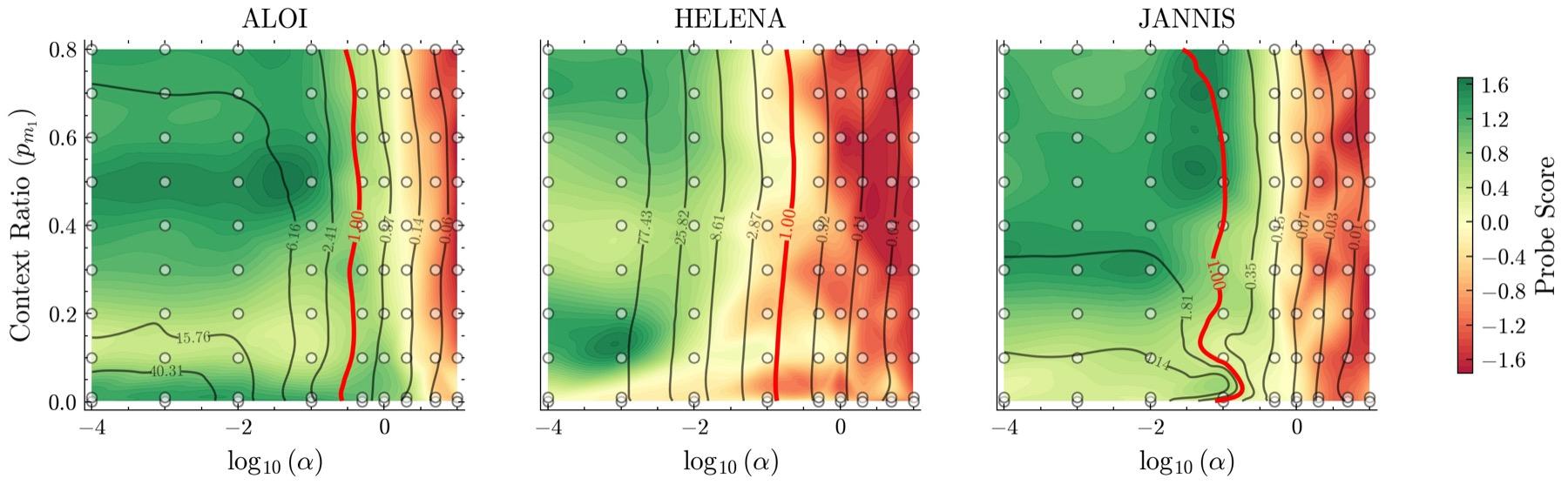
Predictor scale is the strong knob: it divides every μ by α, so it can move any direction across the line. Masking moves the boundary too, by about half a decade with the default spectrum, and the spectrum decides how far. At p = 1 the context is the whole input, every direction has the same data factor, and all the lines meet at α = p_tgt. The paper measured the same plane on three tabular datasets, with a linear-probe score at every point and the μ = 1 contour in red. There too predictor scale does most of the work, and masking bends the boundary, most visibly on jannis at low context ratios:

Three heatmaps (ALOI, HELENA, JANNIS) of normalised linear-probe score over log predictor scale and context ratio, green on the left, red on the right, with a red mu = 1 contour near log alpha between -1.5 and -0.5. — measuredFigure 4 of the paper: sweeps over predictor scale and context ratio on three tabular datasets. Colour is the normalised linear-probe score; the thick red curve is μ = 1.

Cell B sweeps the predictor scale and checks the rank budget of the theory against SGD runs.

Python · B. Sweep the predictor scale

.py

# Cell B. Sweep the predictor scale yourself: theory curve vs SGD runs.
import numpy as np

N, p_tgt, beta, steepness = 10, 1.0, 1.0, 1.2
rng = np.random.default_rng(0)
s0 = 1.0 / np.arange(1, N + 1) ** steepness
R = np.linalg.qr(rng.normal(size=(N, N)))[0]
C = R @ np.diag(s0) @ R.T
C = C / np.sqrt(np.outer(np.diag(C), np.diag(C)))   # unit-diagonal data covariance
s, V = np.linalg.eigh(C)                             # its spectrum is what the theory needs
L = np.linalg.cholesky(C)

def rank_budget(alpha, p):
    mu = p_tgt * s / (alpha * (p * s + 1 - p))
    return int((mu > 1).sum())

def sgd_count(alpha, p, seed=0, batch=256, dt=0.02, t1=2.0, t2=6.0):
    """Train the linear JEPA by SGD and count the directions that grow."""
    rng = np.random.default_rng(seed + 1)
    W = 1e-2 * rng.normal(size=(N, N)); Wa = W.copy(); Wp = alpha * np.eye(N)
    for i in range(int(t2 / dt) + 1):
        x = rng.normal(size=(batch, N)) @ L.T
        x1 = x * (rng.random((batch, N)) < p)
        m2 = rng.random((batch, N)) < p_tgt
        err = (x1 @ W.T) @ Wp.T - m2 * (x @ Wa.T)
        W -= dt * Wp.T @ err.T @ x1 / batch
        Wa += dt * beta * (W - Wa)
        if abs(i * dt - t1) < dt / 2:
            G1 = np.linalg.norm(W @ V, axis=0)
    return int((np.linalg.norm(W @ V, axis=0) > G1).sum())

alphas = np.logspace(-0.6, 0.4, 21)
series = {f"theory, p = {p}": [rank_budget(a, p) for a in alphas] for p in (0.3, 0.7, 0.95)}
plot(np.log10(alphas), series, xlabel="log10 predictor scale", ylabel="rank budget")

print("p = 0.7      alpha   theory   SGD")
for a in alphas[::4]:
    print(f"          {a:6.2f}   {rank_budget(a, 0.7):4d}   {sgd_count(a, 0.7):4d}")

6Seven tricks, one ratio

Practitioners prevent collapse with a collection of devices. The paper takes seven of them and writes each as a term in the linear model (Table 3 and Appendix J). Each acts on μ, through the drive or through the decay, by an amount the paper calls a dose. Pick one and change its dose.

direction (strongest data direction first)

predictor scale α1.00

μ(α) = μ(1) / α

directions that escape

3 of 10

The drive grows like α and the decay like α², so a larger predictor at initialisation pushes every direction toward collapse.

The paper's linear model (10 directions, base predictor scale 1, context keep probability 0.7), with each mechanism written as its derived effect on the decay σ or the drive γ (Table 3 and Appendix J). The paper checks every derived count against 152 simulations of the linear model; all 152 match.

Read across the tabs and the devices sort themselves. Predictor scale and weight decay raise the decay. SIGReg and the VICReg hinge lower the predictor's share of it. The identity predictor takes the predictor out of μ altogether, and the EMA leaves μ untouched. These are statements about the linear model; how each device behaves in a deep network is a separate, empirical question.

Cell C lets you add a device of your own. Write its term in the dynamics and the dose you expect it to have, and the cell checks one against the other. The default is weight decay.

Python · C. Your own mechanism

.py

# Cell C. Add your own anti-collapse mechanism as a term in the dynamics,
# write down its dose on (sigma, gamma), and check the prediction.
import numpy as np

N, p, p_tgt, alpha, beta = 10, 0.7, 1.0, 1.0, 1.0
s = 1.0 / np.arange(1, N + 1) ** 1.2
s = s * N / s.sum()
C = np.diag(s)                                     # unit-diagonal in expectation, eigenbasis = identity
S11 = p * p * C + p * (1 - p) * np.eye(N)          # context auto-covariance under masking
SX1 = p * C                                        # cross-covariance
Wp = alpha * np.eye(N)

eta = 0.15   # <- the dose

def extra(W):
    """Your mechanism, as an extra term in dW/dt. Default: encoder weight decay."""
    return -eta * W

def dose(sigma, gamma):
    """What the mechanism does to one direction. Weight decay adds a floor to the decay."""
    return sigma + eta, gamma

# Prediction from the dose
sigma = alpha**2 * np.diag(S11)
gamma = alpha * p_tgt * np.diag(SX1)
sig2, gam2 = dose(sigma, gamma)
print("escape without the mechanism:", int((gamma / sigma > 1).sum()), "of", N)
print("escape with it, predicted:   ", int((gam2 / sig2 > 1).sum()), "of", N)

# Measurement: integrate the expected flow (Lemma 3.1) with the extra term
rng = np.random.default_rng(0)
W = 1e-2 * rng.normal(size=(N, N)); Wa = W.copy(); dt = 0.01
for i in range(800):
    if i == 200:
        G1 = np.linalg.norm(W, axis=0)
    dW = -Wp.T @ Wp @ W @ S11 + p_tgt * Wp.T @ Wa @ SX1.T + extra(W)
    W, Wa = W + dt * dW, Wa + dt * beta * (W - Wa)
print("escape with it, measured:    ", int((np.linalg.norm(W, axis=0) > G1).sum()), "of", N)

7Fix it with the identity

If a large predictor pushes μ down, start from a predictor that does nothing. Write it as the identity plus a correction that starts at zero, W_p = I + ΔW_p. Then the predictor factor is set by the target mask alone, and μ no longer depends on how the predictor was initialised:

μ_{k} = \frac{p_{tgt} s_{k}}{p s_{k} + 1 - p}

A transformer predictor is not a matrix, but its attention can start as one. ResidualPred adds a bias on the diagonal of the attention logits,

Attention (Q, K, V) = softmax (\frac{Q K^{⊤}}{\sqrt{d}} + β_{init} \cdot I) V

so that at initialisation every token attends to itself. Raise the bias and watch the grey turn into a diagonal.

row: query tokencolumn: attended token

diagonal bias β_init0.0

saturation bound log n + 5 = 7.5

smallest self-attention Aᵢᵢ

0.057

effective rank of A

3.3 of 12

One attention head at initialisation: 12 context tokens, queries and keys at the scale of a standard initialisation (logit standard deviation about 0.16), softmax(QKᵀ/√d + β_init·I). The threshold log n + 5 is the paper's saturation bound (Appendix D); the paper uses β_init = 10.

Without the bias, attention at initialisation is close to uniform: every token receives nearly the same average of the others, so the differences between tokens are washed out, and the effective rank of the attention matrix is a fraction of the number of tokens. Near log n + 5 every self-weight reaches 0.99 and the matrix is the identity. The paper uses β_init = 10 everywhere. In the released code the bias is a learnable parameter, one per head, on the diagonal of the context block. It adds no loss term and no cost per step.

The identity is where the predictor starts, not where it should stay. Frozen at initialisation and denied learning, the ResidualPred predictor collapses the representation (Section 6.2).

Python · D. ResidualPred's attention in numpy

.py

# Cell D. ResidualPred's attention at initialisation, in numpy.
import numpy as np

def attention(Q, K, V, beta_init):
    """softmax(Q K^T / sqrt(d) + beta_init * I) V, the diagonal-bias attention of ResidualPred."""
    n, d = Q.shape
    logits = Q @ K.T / np.sqrt(d) + beta_init * np.eye(n)
    A = np.exp(logits - logits.max(axis=1, keepdims=True))
    A /= A.sum(axis=1, keepdims=True)
    return A @ V, A

rng = np.random.default_rng(0)
n, d = 54, 32          # 54 context tokens, as on CIFAR with keep probability 0.85
Q, K = 0.4 * rng.normal(size=(2, n, d))   # a standard initialisation: logits with std about 0.16
V = rng.normal(size=(n, d))
print("beta_init   min A_ii   output = input?")
for b in (0, 2, 5, np.log(n) + 5, 10):
    out, A = attention(Q, K, V, b)
    print(f"{b:8.2f}   {A.diagonal().min():.4f}     max |out - V| = {np.abs(out - V).max():.3f}")

# In the released code the bias sits on the diagonal of the context block only (the target tokens
# appended after the context attend freely), and it is a learnable parameter, one per head.
n_ctx, n_tgt = 54, 10
Qa, Ka = 0.4 * rng.normal(size=(2, n_ctx + n_tgt, d))
bias = np.zeros((n_ctx + n_tgt, n_ctx + n_tgt)); bias[:n_ctx, :n_ctx] = np.eye(n_ctx)
logits = Qa @ Ka.T / np.sqrt(d) + 10.0 * bias
A = np.exp(logits - logits.max(axis=1, keepdims=True)); A /= A.sum(axis=1, keepdims=True)
print(f"context rows: min A_ii = {A[:n_ctx].diagonal().min():.4f};  target rows: max weight = {A[n_ctx:].max():.3f}")

8Beyond the linear model

Everything so far is the linear model. The results on deep networks are measurements, and the paper keeps the two apart. ResidualPred was dropped into I-JEPA on images, with the encoder and the training recipe unchanged.

I-JEPA, standard predictor+ ResidualPred

Table view

Dataset	I-JEPA	+ ResidualPred
CIFAR-10	64.55 ± 1.71	68.61 ± 0.59
CIFAR-100	36.83 ± 1.49	40.85 ± 0.66
STL-10	71.25 ± 1.14	75.31 ± 0.78
ImageNet-100	37.09 ± 0.68	42.73 ± 0.41
ImageNet-1k pilot*	25.22 ± 0.80	31.69 ± 0.22

Linear-probe accuracy of I-JEPA with the standard predictor and with ResidualPred, mean over seeds with ± one standard deviation (paper, Table 4; ImageNet-1k from Table 5). *ImageNet-1k: a pilot at a matched 30-epoch budget, ViT-S/16, five seeds per arm; tripling the schedule to 90 epochs attenuates the margin.

On the ImageNet-1k pilot, ResidualPred also compares well with SIGReg, the regulariser of LeJEPA, and the two combine (Table 5, five seeds each):

ImageNet-1k pilot	Linear probe (%)	Effective rank
I-JEPA	25.22 ± 0.80	107.2 ± 7.7
+ SIGReg	29.19 ± 0.54	185.6 ± 5.6
+ ResidualPred	31.69 ± 0.22	188.5 ± 3.3
+ ResidualPred + SIGReg	32.23 ± 0.54	206.7 ± 1.0

Proven

In linear networks with spectral decoupling: the μ > 1 criterion, the rank budget, and the dose of each of the seven mechanisms. Near collapse the criterion also holds with the predictor trained jointly.

Measured

The phase boundary across more than 800 Tabular-JEPA configurations, and the gains of ResidualPred on images. Whether μ is what carries those gains in deep networks is not established: at initialisation a whole-block estimator does not separate the two predictors, and the first link of the mechanism is measured after a few predictor-only steps, in 9 of 9 matched comparisons.

9Cheat sheet

My JEPA's loss went to zero. Is that good news?: Not by itself. The collapsed solution has zero loss too. Track the effective rank of the embeddings. See chapter 1
Will a slower EMA prevent collapse?: In the linear model, no. β changes how fast directions grow or die, never which ones. See chapter 3
How large should the predictor be at initialisation?: Small enough that μ > 1 for the directions you want to keep. μ scales like 1/α. See chapter 4
Does more masking help?: It depends on the spectrum of the data. In the linear model, masking moves the strong and the weak directions in opposite ways. See chapter 4
Should I add SIGReg or VICReg?: In the linear model both lower the predictor's share of the decay, which raises μ. On the ImageNet-1k pilot, SIGReg and ResidualPred stack. See chapter 6
What is the cheapest change to try?: Start the predictor's attention at the identity: one hyperparameter, β_init = 10, no extra loss term and no per-step cost. See chapter 7

Run it for real

The four cells are also a notebook: drive_vs_decay_tutorial.ipynb (numpy and matplotlib only). The experiments of the paper, tabular and image, are in the code repository.

Paper (arXiv)Project page and video